
Amazon SageMaker and Jupyter Notebooks: From Console to Your First Dataset
A walkthrough of the classic AWS guided lab: launch a SageMaker notebook instance, explore JupyterLab, run sample notebooks, and download the Vertebral Column medical dataset into pandas—so you have a reproducible starting point for later ML exercises.
In short
SageMaker gives you managed Jupyter on EC2. You create a notebook instance, open JupyterLab, mix Markdown and code cells, and pull external data into a DataFrame. Stop or delete the instance when the lab ends so you are not billed for idle compute.
Why SageMaker and Jupyter together
Amazon SageMaker is AWS’s managed machine learning platform. It covers the full ML lifecycle—data prep, training, tuning, deployment, and monitoring—without you operating every server by hand. For learning and experimentation, the entry point most people remember is the notebook instance: a preconfigured EC2 host that runs JupyterLab, with conda environments for common frameworks (TensorFlow, PyTorch, scikit-learn, and more).
Jupyter notebooks are documents that mix narrative (Markdown), code, and output in one place. You run cells in order; each execution gets a number like In[8] so you can see what ran when. That model fits exploration: try a plot, adjust a parameter, document the reasoning in the cell above. Official references: jupyter.org, the Jupyter Notebook documentation, and a beginner-friendly overview at DataCamp’s Jupyter tutorial.
If you already have vocabulary from Machine Learning Foundations or the AI/ML glossary, this lab is where those ideas meet a real keyboard: features, labels, and a tabular dataset loaded in pandas.
Task 1 — Create a SageMaker notebook instance
In the AWS Management Console, search for Amazon SageMaker AI (the console name may show “SageMaker” depending on region and UI version). From the left navigation, open Notebooks and choose Create notebook instance.
| Setting | Lab value | Why it matters |
|---|---|---|
| Notebook instance name | MyNotebook | Identifies the instance in the console and in IAM/resource tags. |
| Instance type | ml.m4.xlarge | CPU/RAM sized for interactive notebooks; labs often use a modest instance. |
| Platform identifier | notebook-al2-v3 | Amazon Linux 2 base image—current default for many notebook AMIs. |
| Lifecycle configuration | Configuration containing ml-pipeline | Runs a startup script that copies sample notebooks (e.g. cheat sheets, MNIST sample) into your home directory. |
Leave other options at their defaults unless your organization requires a VPC, encryption key, or specific IAM role. Choose Create notebook instance. Status moves from Pending to InService in roughly two to five minutes. When it is ready, choose Open JupyterLab at the end of the row.
Cost habit: A running notebook instance bills for the underlying EC2 hours. When you finish a lab, Stop the instance if you might return soon, or Delete it when you are done. Stopped storage may still incur a small charge; deleted instances do not.
Task 2 — JupyterLab layout and cell types
JupyterLab is the modern multi-tab IDE. The menu bar groups commands you will use often:
- File — save, revert, checkpoints.
- Edit — cut, copy, paste, delete cells (dd deletes a cell in command mode).
- Run — execute one or many cells.
- Kernel — restart or change the Python environment (TensorFlow, PyTorch, plain conda, etc.).
- Git — version control when a repo is configured.
On the left, the sidebar holds the file browser, running kernels/terminals, command palette, table of contents for headings, and SageMaker sample listings. The main area is tabbed: drag tabs to split panes horizontally or vertically. The active tab shows a colored top border.
Each notebook has a toolbar when focused: save, insert/cut/copy/paste, run/interrupt/restart, a cell type dropdown, and the kernel name (for example conda_python3 or conda_python310).
Cell types and how to run them
- Code — Python (or another kernel language); output appears below the cell.
- Markdown — headings, lists, links; rendered as formatted HTML when you run the cell.
- Raw — passed through without execution (export tooling).
Run the focused cell with Shift+Enter, the toolbar run button, or Run → Run Selected Cells. In command mode (press Esc), press M to change the cell to Markdown and Y to change it back to code.
Open the lifecycle-provided PythonCheatSheet.ipynb from the language folder in the file browser. Double-click the first Markdown cell to see raw Markdown (e.g. # for headings). Run through the notebook once: Markdown cells render documentation; code cells execute and show In[n] / Out[n] numbering. That numbering is your audit trail—if results look wrong, check whether cells were run out of order.
Task 3 — Sample notebook (read-only exploration)
In the same folder, open linear_learner_mnist.ipynb. Use Create a Copy in the header so you edit your own copy, not the read-only original. Scroll through the notebook to see how a full SageMaker workflow is structured: data in S3, training job, endpoint. You typically cannot run every step in a short lab without your own S3 bucket and IAM permissions—the sample assumes AWS resources that a sandbox may not grant. Treat it as architecture reading, not a mandatory execution checklist.
Task 4 — New notebook and import the Vertebral Column data
For the rest of the guided labs you need a clean notebook and a shared dataset. The Vertebral Column dataset (UCI Machine Learning Repository) contains biomechanical features used to classify spine conditions—useful for supervised classification practice.
Create the notebook and title cell
- File → New → Notebook.
- In Select kernel, choose
conda_python310(labs may also offerconda_python3; match what your environment lists). - Press M to set the first cell to Markdown, type
# Importing the data, then Shift+Enter to render it.
Download and extract the ZIP in memory
Instead of saving a ZIP to disk manually, stream it with requests and extract with zipfile:
import warnings, requests, zipfile, io
warnings.simplefilter('ignore')
import pandas as pd
from scipy.io import arff

f_zip = 'http://archive.ics.uci.edu/ml/machine-learning-databases/00212/vertebral_column_data.zip'
r = requests.get(f_zip, stream=True)
Vertebral_zip = zipfile.ZipFile(io.BytesIO(r.content))
Vertebral_zip.extractall()
Add the import cell, press B to insert a cell below for the download block, then select both code cells and run with Shift+Enter. In the file browser you should see four extracted files:
column_2C_weka.arff/column_2C.dat— two classes (e.g. normal vs abnormal).column_3C_weka.arff/column_3C.dat— three classes.
Open the .dat files in the editor: they are plain text, often space- or tab-separated, sometimes without a header row in the raw file. The .arff format is Weka’s attribute-relation format: it declares attribute names and types in a header, then lists instances—ideal for loading into pandas via SciPy.
Load ARFF into a DataFrame
data = arff.loadarff('column_2C_weka.arff')
df = pd.DataFrame(data[0])
df.head()
After you run this cell, head() shows the first rows. Expect columns such as pelvic incidence, pelvic tilt, lumbar lordosis angle, sacral slope, pelvic radius, degree of spondylolisthesis, and class. ARFF may store string labels as byte strings (e.g. b'Abnormal'); for modeling you will often decode or map them to categories in a later step.
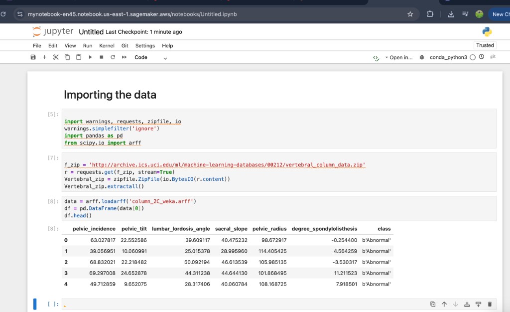
df.head() on the two-class Vertebral Column file.What you learned in this step
- External data can enter the notebook with a URL and a few lines of Python—no manual download step on your laptop.
- File format matters: ARFF carries schema metadata; raw
.datfiles need you to infer or look up column names. - pandas is the usual bridge from “files on the notebook instance” to “tables you can plot and model.”
Task 5 — Save your work (optional but recommended)
Lab sandboxes are ephemeral: when the environment ends, the notebook instance and local files are destroyed unless you saved them elsewhere.
- In the JupyterLab file browser, right-click your notebook → Download to keep a
.ipynbon your machine. - For team or long-term storage, copy notebooks and data to Amazon S3 or commit to Git (excluding large datasets and secrets).
- On a future lab, recreate the notebook instance, upload the file, and re-run cells—or automate setup with a lifecycle script.
Jupyter shortcuts worth memorizing
| Mode | Keys | Action |
|---|---|---|
| Command | Esc | Leave edit mode |
| Command | A / B | Insert cell above / below |
| Command | M / Y | Markdown / code cell |
| Command | dd | Delete cell |
| Any | Shift+Enter | Run cell and advance |
From this lab to production ML on AWS
Notebooks are for exploration; production paths usually add S3 for datasets, SageMaker training jobs for repeatable training, model registry for versions, and endpoints or batch transform for inference. Studio and SageMaker Pipelines extend the same ideas with CI/CD-friendly workflows—topics covered in depth in MLA-C01 practice material and how to become an AI developer.
For generative workloads, many teams now start in Amazon Bedrock; for custom classical or deep models, SageMaker remains the default managed path on AWS.
Lab checklist
- Notebook instance InService, JupyterLab opened.
- Explored PythonCheatSheet and skimmed MNIST sample copy.
- New notebook with Markdown title and vertebral data loaded into
df. - Downloaded notebook if you need it after the lab ends.
- Stopped or deleted the notebook instance to avoid unnecessary charges.
Blog index · ML Foundations · Supervised vs unsupervised vs RL